mt_plot can be used for plotting a number of individual trajectories.
mt_plot_aggregate can be used for plotting aggregated trajectories.
The color and linetype can be varied depending on a set of condition
variables using the color and linetype arguments. If the
x and y arguments are varied, this function can also be used
for plotting velocity and acceleration profiles.
mt_plot(
  data,
  use = "trajectories",
  use2 = "data",
  x = "xpos",
  y = "ypos",
  color = NULL,
  linetype = NULL,
  alpha = NA,
  size = 0.5,
  facet_row = NULL,
  facet_col = NULL,
  wrap_var = NULL,
  wrap_ncol = NULL,
  points = FALSE,
  return_type = "plot",
  mt_id = "mt_id",
  only_ggplot = NULL,
  ...
)

mt_plot_aggregate(
  data,
  use = "trajectories",
  use2 = "data",
  x = "xpos",
  y = "ypos",
  color = NULL,
  linetype = NULL,
  alpha = NA,
  size = 0.5,
  facet_row = NULL,
  facet_col = NULL,
  wrap_var = NULL,
  wrap_ncol = NULL,
  points = FALSE,
  return_type = "plot",
  subject_id = NULL,
  only_ggplot = NULL,
  ...
)
Arguments
- data
a mousetrap data object created using one of the mt_import functions (see mt_example for details). Alternatively, a trajectory array can be provided directly (in this case
usewill be ignored).- use
a character string specifying which trajectories should be plotted. The corresponding trajectories are selected from data using
data[[use]]. Usually, this value corresponds to either "trajectories", "tn_trajectories" or "av_trajectories", depending on whether the raw, time-normalized or averaged trajectories should be plotted.- use2
a character string specifying where the data that contain the variables used for determining the
colorandlinetypecan be found (in case these arguments are specified). Defaults to "data" asdata[["data"]]usually contains all non mouse-tracking trial data.- x
a character string specifying which dimension in the trajectory array should be displayed on the x-axis (defaults to xpos).
- y
a character string specifying which dimension in the trajectory array should be displayed on the y-axis (defaults to ypos).
- color
an optional character string specifying which variable in
data[[use2]]should be used for coloring the trajectories.- linetype
an optional character string specifying which variable in
data[[use2]]should be used for varying the linetype of the trajectories.- alpha
an optional numeric value between 0 and 1 that can be used to make the plotted lines (and points) semitransparent.
- size
an optional numeric value that can be used to vary the width of the plotted trajectory lines.
- facet_row
an optional character string specifying a variable in
data[[use2]]that should be used for (row-wise) faceting.- facet_col
an optional character string specifying a variable in
data[[use2]]that should be used for (column-wise) faceting.- wrap_var
an optional character string specifying variable(s) in
data[[use2]]that should be used for wrapping.- wrap_ncol
an optional integer specifying the number of columns if wrapping is used.
- points
logical. If
TRUE, points will be added to the plot using geom_point.- return_type
a character string specifying which type of object should be returned. If
"plot"(the default), a new ggplot is created and the trajectories are plotted using geom_path. If"mapping", only the ggplot object containing the mapping but without any geoms is returned. If"geoms", only the geoms are returned, which allows adding the plotted trajectories to an existing ggplot.- mt_id
a character string specifying the internal label used for the trial identifier (passed on to the group aesthetic). Only relevant for
mt_plot.- only_ggplot
Deprecated. Please use
return_typeinstead.- ...
additional arguments passed on to mt_reshape (such as
subset).- subject_id
a character string specifying which column contains the subject identifier. Only relevant for
mt_plot_aggregate. If specified, aggregation will be performed within subjects first. Note that aggregation will be performed separately for each level, including all subjects for whom data are available.
Details
mt_plot internally uses mt_reshape for reshaping trajectories
into a long format. Next, it creates a ggplot object using the
ggplot function of the ggplot2 package. The
aes mappings are taken from the function arguments for x, y
etc.; in addition, the group mapping is set to the internal trial identifier
(by default called "mt_id").
If return_type == "plot" (the default), a new ggplot is created and
the trajectories are plotted using the geom_path function of
the ggplot2 package. If return_type == "mapping", the ggplot
object is returned without layers, which can be used to further customize the
plot (see Examples). If return_type == "geoms", only the geoms are
returned, which allows adding the plotted trajectories to an existing ggplot
(e.g., adding aggregate trajectories on top of the individual trajectories,
see Examples).
mt_plot_aggregate works similarly, but uses mt_aggregate for
reshaping and aggregating trajectories prior to plotting.
Please note that this function is intended as a quick and easy solution for visualizing mouse trajectories. For additional flexibility, we recommend that mt_reshape or mt_aggregate be used in conjunction with ggplot to create custom visualizations.
Functions
mt_plot(): Plot individual trajectory datamt_plot_aggregate(): Plot aggregated trajectory data
See also
mt_plot_add_rect for adding rectangles representing the response buttons to the plot.
mt_plot_riverbed for plotting the relative frequency of a selected variable across time.
mt_plot_per_trajectory for individually plotting all trajectories as individual pdf files.
Examples
## Plot individual example trajectories
# Time-normalize trajectories
mt_example <- mt_time_normalize(mt_example)
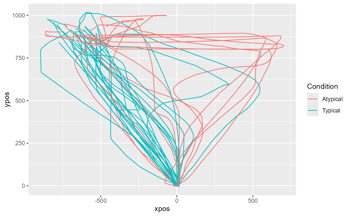
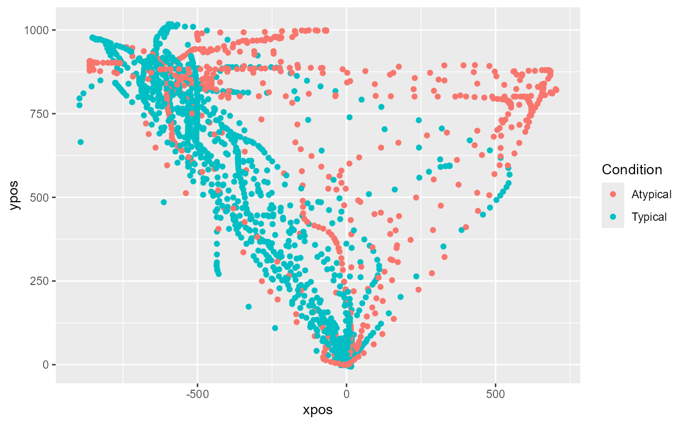
# Plot all time-normalized trajectories
# varying the color depending on the condition
mt_plot(mt_example, use="tn_trajectories",
color="Condition")
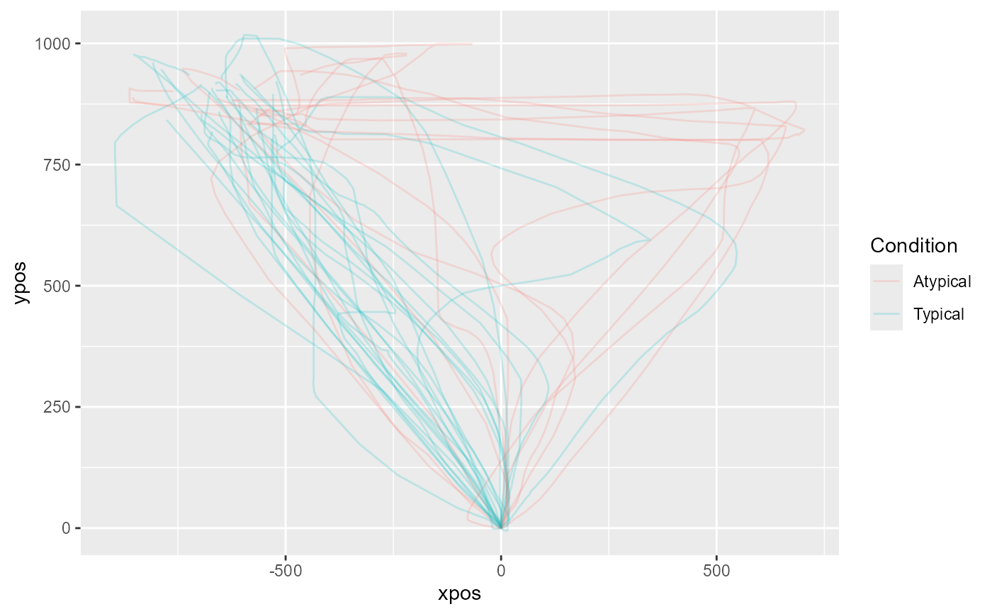
 # ... setting alpha < 1 for semi-transparency
mt_plot(mt_example, use="tn_trajectories",
color="Condition", alpha=.2)
# ... setting alpha < 1 for semi-transparency
mt_plot(mt_example, use="tn_trajectories",
color="Condition", alpha=.2)
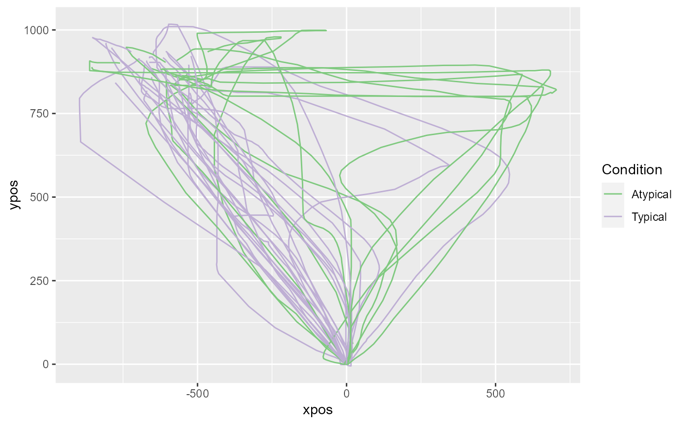
 # ... with custom colors
mt_plot(mt_example, use="tn_trajectories",
color="Condition") +
ggplot2::scale_color_brewer(type="qual")
# ... with custom colors
mt_plot(mt_example, use="tn_trajectories",
color="Condition") +
ggplot2::scale_color_brewer(type="qual")
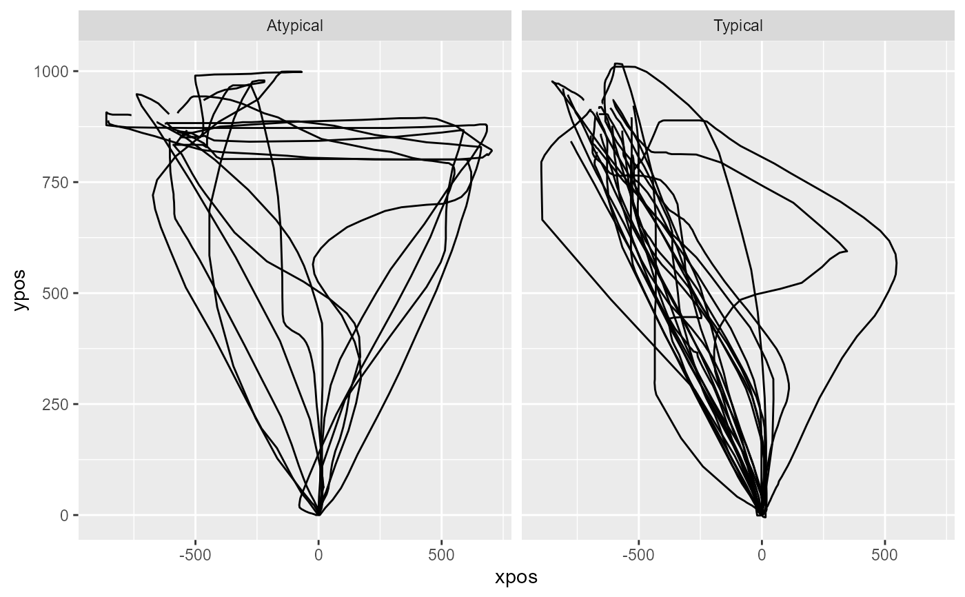
 # Create separate plots per Condition
mt_plot(mt_example, use="tn_trajectories",
facet_col="Condition")
# Create separate plots per Condition
mt_plot(mt_example, use="tn_trajectories",
facet_col="Condition")
 # Create customized plot by setting the return_type option to "mapping"
# to setup an empty plot. In a next step, a geom is added.
# In this example, only points are plotted.
mt_plot(mt_example, use="tn_trajectories",
color="Condition", return_type="mapping") +
ggplot2::geom_point()
# Create customized plot by setting the return_type option to "mapping"
# to setup an empty plot. In a next step, a geom is added.
# In this example, only points are plotted.
mt_plot(mt_example, use="tn_trajectories",
color="Condition", return_type="mapping") +
ggplot2::geom_point()
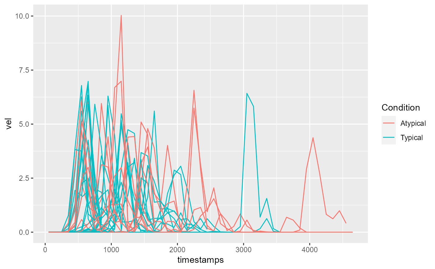
 # Plot velocity profiles based on the averaged trajectories
# varying the color depending on the condition
mt_example <- mt_derivatives(mt_example)
mt_example <- mt_average(mt_example, interval_size=100)
mt_plot(mt_example, use="av_trajectories",
x="timestamps", y="vel", color="Condition")
# Plot velocity profiles based on the averaged trajectories
# varying the color depending on the condition
mt_example <- mt_derivatives(mt_example)
mt_example <- mt_average(mt_example, interval_size=100)
mt_plot(mt_example, use="av_trajectories",
x="timestamps", y="vel", color="Condition")
 ## Plot aggregate trajectories for KH2017 data
# Time-normalize trajectories
KH2017 <- mt_time_normalize(KH2017)
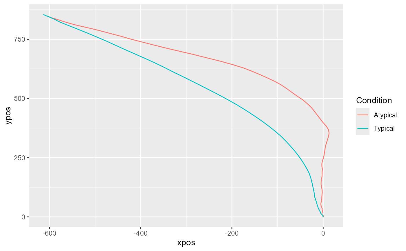
# Plot aggregated time-normalized trajectories per condition
mt_plot_aggregate(KH2017, use="tn_trajectories",
color="Condition")
## Plot aggregate trajectories for KH2017 data
# Time-normalize trajectories
KH2017 <- mt_time_normalize(KH2017)
# Plot aggregated time-normalized trajectories per condition
mt_plot_aggregate(KH2017, use="tn_trajectories",
color="Condition")
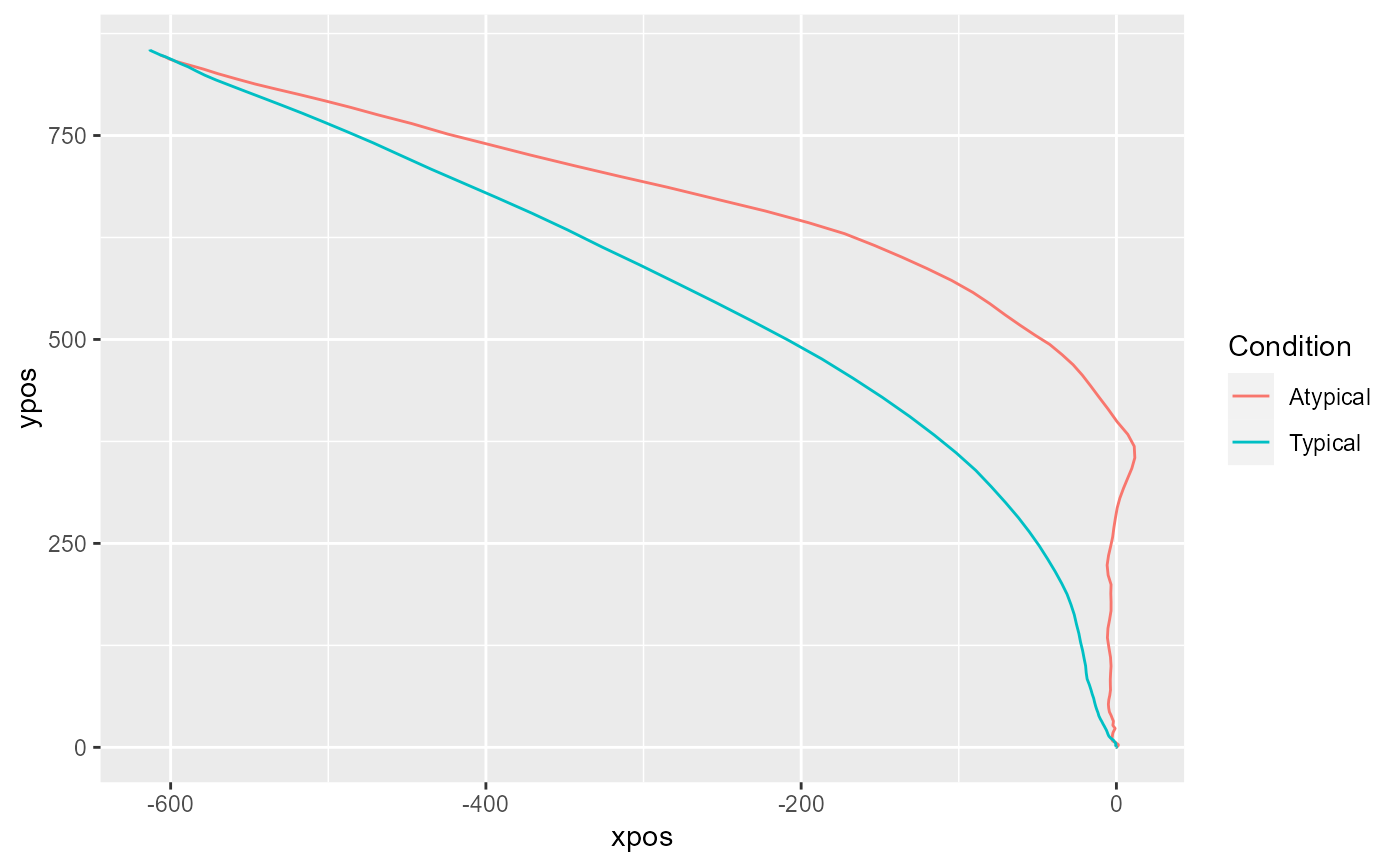
 # ... first aggregating trajectories within subjects
mt_plot_aggregate(KH2017, use="tn_trajectories",
color="Condition", subject_id="subject_nr")
# ... first aggregating trajectories within subjects
mt_plot_aggregate(KH2017, use="tn_trajectories",
color="Condition", subject_id="subject_nr")
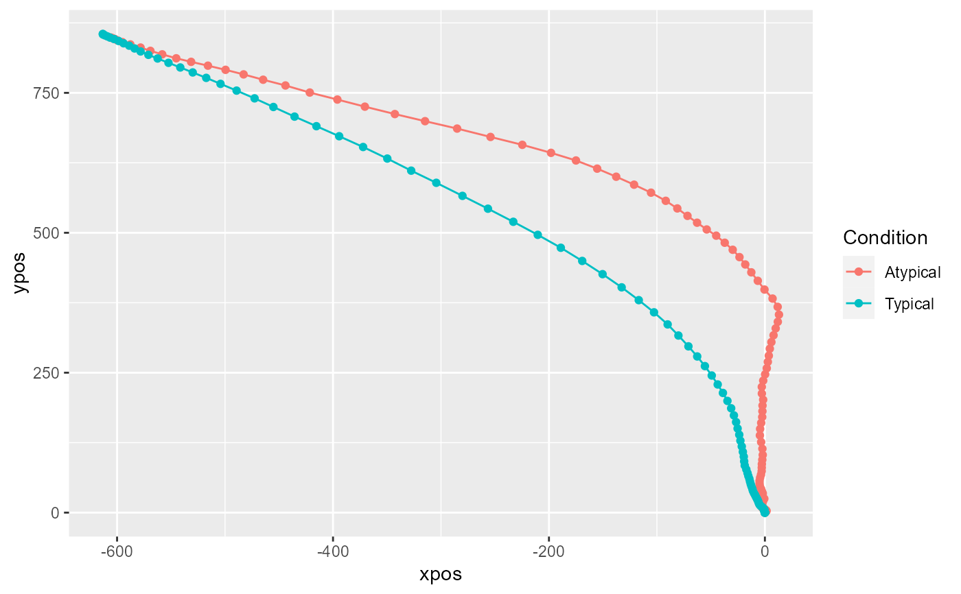
 # ... adding points for each position to the plot
mt_plot_aggregate(KH2017, use="tn_trajectories",
color="Condition", points=TRUE)
# ... adding points for each position to the plot
mt_plot_aggregate(KH2017, use="tn_trajectories",
color="Condition", points=TRUE)
 if (FALSE) { # \dontrun{
# Create combined plot of individual and aggregate trajectories
# by first plotting the individual trajectories using mt_plot.
# In a next step, the aggregate trajectories are added using the
# mt_plot_aggregate function with the return_type argument set to "geom".
mt_plot(KH2017, use="tn_trajectories", color="Condition", alpha=.05) +
mt_plot_aggregate(KH2017, use="tn_trajectories",
color="Condition", return_type="geom", size=2)
} # }
if (FALSE) { # \dontrun{
# Create combined plot of individual and aggregate trajectories
# by first plotting the individual trajectories using mt_plot.
# In a next step, the aggregate trajectories are added using the
# mt_plot_aggregate function with the return_type argument set to "geom".
mt_plot(KH2017, use="tn_trajectories", color="Condition", alpha=.05) +
mt_plot_aggregate(KH2017, use="tn_trajectories",
color="Condition", return_type="geom", size=2)
} # }