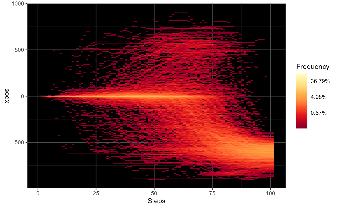
mt_plot_riverbed creates a plot showing the distribution of one
trajectory variable (e.g., the x-positions or velocity) per time step.
mt_plot_riverbed(
  data,
  use = "tn_trajectories",
  y = "xpos",
  y_range = NULL,
  y_bins = 250,
  facet_row = NULL,
  facet_col = NULL,
  facet_data = "data",
  grid_colors = c("gray30", "gray10"),
  na.rm = FALSE
)
Arguments
- data
mousetrap data object containing the data to be plotted.
- use
character string specifying the set of trajectories to use in the plot. The steps of this set will constitute the x axis. Defaults to 'tn_trajectories', which results in time steps being plotted on the x axis.
- y
variable in the mousetrap data object to be plotted on the output's y dimension. Defaults to 'xpos', the cursor's x coordinate.
- y_range
numerical vector containing two values that represent the upper and lower ends of the y axis. By default, the range is calculated from the data provided.
- y_bins
number of bins to distribute along the y axis (defaults to 250).
- facet_row
an optional character string specifying a variable in
data[[facet_data]]that should be used for (row-wise) faceting. If specified, separate riverbed plots for each level of the variable will be created.- facet_col
an optional character string specifying a variable in
data[[facet_data]]that should be used for (column-wise) faceting. If specified, separate riverbed plots for each level of the variable will be created.- facet_data
a character string specifying where the (optional) data containing the faceting variables can be found.
- grid_colors
a character string or vector of length 2 specifying the grid color(s). If a single value is provided, this will be used as the grid color. If a vector of length 2 is provided, the first value will be used as the color for the major grid lines, the second value for the minor grid lines. If set to
NA, no grid lines are plotted.- na.rm
logical specifying whether missing values should be removed. This is not done by default, because generally riverbed plots are generated from preprocess trajectories (e.g., time-normalized trajectories) that all have the same length (i.e., the same number of steps).
Details
This function plots the relative frequency of the values of a trajectory variable separately for each of a series of time steps. This type of plot has been used in previous research to visualize the distribution of x-positions per time step (e.g., Scherbaum et al., 2010).
mt_plot_riverbed usually is applied to time-normalized trajectory data
as all trajectories must contain the same number of values (if
na.rm=FALSE, the default).
References
Scherbaum, S., Dshemuchadse, M., Fischer, R., & Goschke, T. (2010). How decisions evolve: The temporal dynamics of action selection. Cognition, 115(3), 407-416.
Scherbaum, S., & Kieslich, P. J. (2018). Stuck at the starting line: How the starting procedure influences mouse-tracking data. Behavior Research Methods, 50(5), 2097–2110.
See also
mt_plot for plotting trajectory data.
mt_time_normalize for time-normalizing trajectories.
Examples
# Time-normalize trajectories
KH2017 <- mt_time_normalize(KH2017)

# Create riverbed plot for all trials
mt_plot_riverbed(KH2017)


if (FALSE) { # \dontrun{
# Create separate plots for typical and atypical trials
mt_plot_riverbed(mt_example, facet_col="Condition")


# Create riverbed plot for all trials with custom x and y axis labels
mt_plot_riverbed(mt_example) +
  ggplot2::xlab("Time step") + ggplot2::ylab("X coordinate")

# Note that it is also possible to replace the
# default scale for fill with a custom scale
mt_plot_riverbed(mt_example, facet_col="Condition") +
  ggplot2::scale_fill_gradientn(colours=grDevices::heat.colors(9),
    name="Frequency", trans="log", labels=scales::percent)
} # }
if (FALSE) { # \dontrun{
# Create separate plots for typical and atypical trials
mt_plot_riverbed(mt_example, facet_col="Condition")
# Create riverbed plot for all trials with custom x and y axis labels
mt_plot_riverbed(mt_example) +
ggplot2::xlab("Time step") + ggplot2::ylab("X coordinate")
# Note that it is also possible to replace the
# default scale for fill with a custom scale
mt_plot_riverbed(mt_example, facet_col="Condition") +
ggplot2::scale_fill_gradientn(colours=grDevices::heat.colors(9),
name="Frequency", trans="log", labels=scales::percent)
} # }